Problem1 - b, c
Consider the case when \(H=W\) (a square cavity). Here, the Reynolds number, \(Re=UW/\nu\), characterizes the flow patters. Compute the steady state solutions for both \(Re=100\) and \(Re=500\). Plot the flow streamlines and centerline profiles (\(u\) vs. \(y\) and \(v\) vs. \(x\) through the center of the domain). For \(Re=100\), valdiate your method by comparing your results to data from given literature.
Re = 100
In this test, the lid cavity’s velocity is set to make the Reynolds number set to 100. To see the qualitative effect of different grid spacing, four different grid resolution conditions is employed and compared together in this page.
- NxN = 10x10
<Streamlines of 10x10 case runs>

<Centerline u-velocity compared with Ghia’s numerically resolved data>

<Centerline v-velocity compared with Ghia’s numerically resolved data>
- Observation
- Very coarse grid resolution doesn’t produce well-predicted data when it is compared to the reference data.
- Even though the streamlines seems to penetrate the wall, it does not necessarily mean it pass through it. It it because the default streamline generation feature of Python does not produce properly when it is resolved on less grid points.
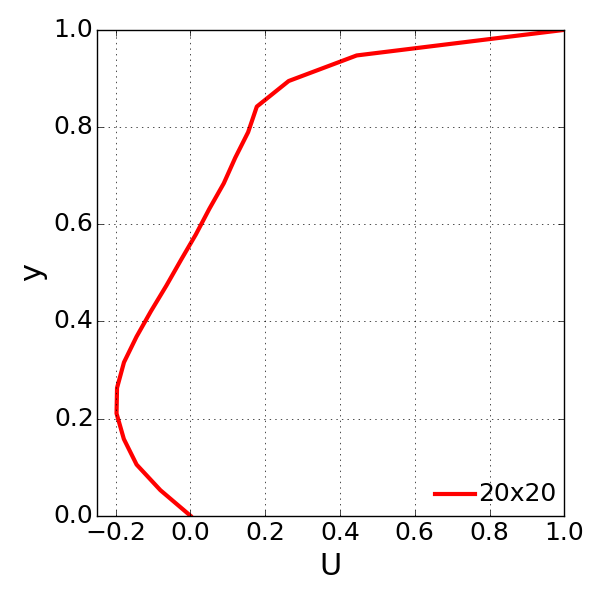
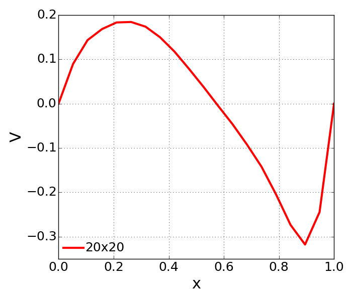
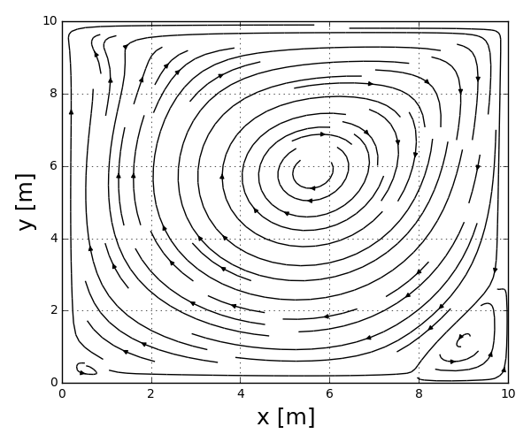
- NxN = 20x20
<Streamlines of 20x20 case runs>
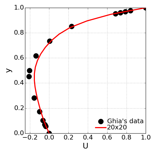
<Centerline u-velocity compared with Ghia’s numerically resolved data>
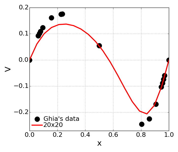
<Centerline v-velocity compared with Ghia’s numerically resolved data>
- Observation
- Denser grid resolution tends to produce better results. The resolved u and v velocities look closer to the reference data.
- Compared to 10x10 case, the streamline produced with denser grid resolution looks more physically reasonable.
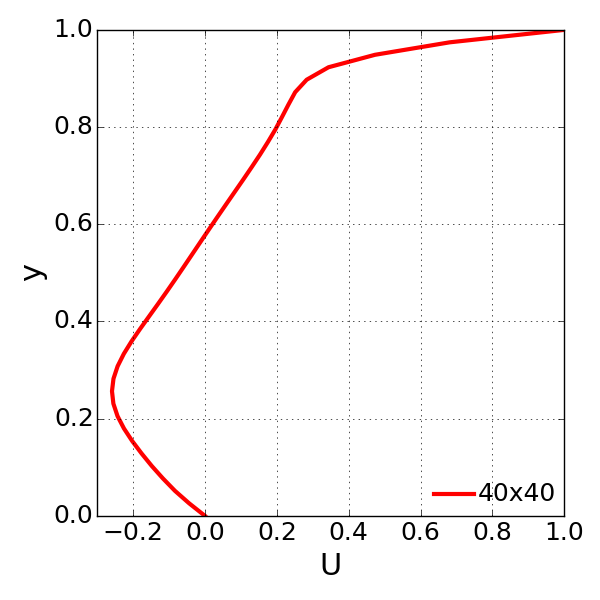
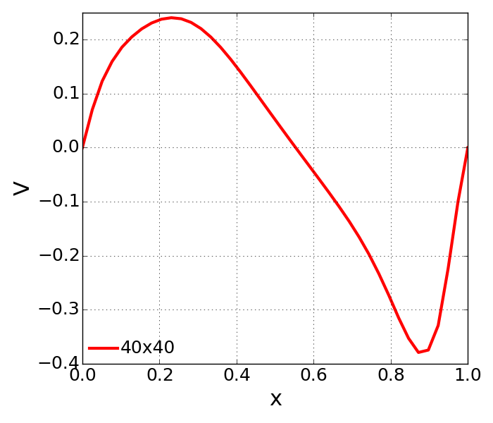
- NxN = 40x40
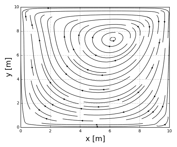
<Streamlines of 40x40 case runs>

<Centerline u-velocity compared with Ghia’s numerically resolved data>
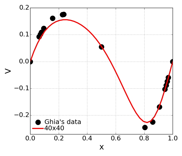
<Centerline v-velocity compared with Ghia’s numerically resolved data>
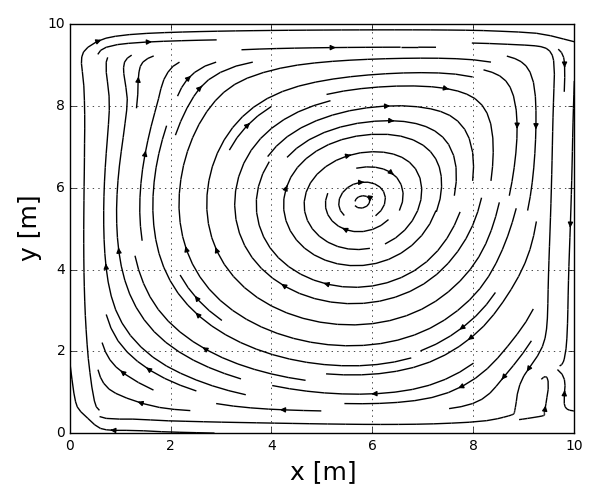
- NxN = 60x60
<Streamlines of 60x60 case runs>

<Centerline u-velocity compared with Ghia’s numerically resolved data>

<Centerline v-velocity compared with Ghia’s numerically resolved data>
- Observation
- Having resolution of 60x60 makes finally the resolved data looks very close to the reference data.
- We observed the denser grid size produces the more well-matching data with reference data.
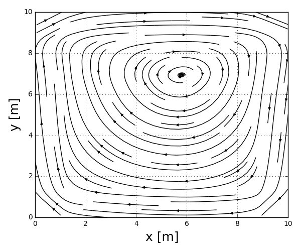
Re = 500
In this test, the lid cavity velocity is set to 50 m/s to make the Reynolds number 500. Two different grid spacing are employed to see the qualitative pattern of grid size effect on numerical solution.
- NxN = 20x20
<Streamlines of 20x20 case runs>
<Centerline u-velocity>
<Centerline v-velocity>
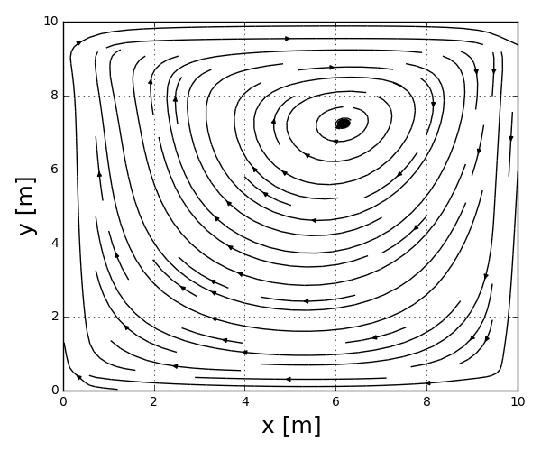
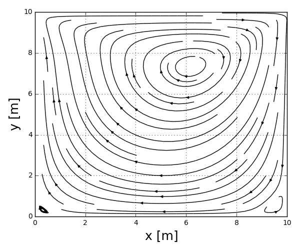
- NxN = 40x40
<Streamlines of 40x40 case runs>
<Centerline u-velocity>
<Centerline v-velocity>
- Observation
- The faster lid cavity velocity makes the distictive vortex at two corners on the bottom where as Re=100 case produces very weak vortext at the same location.
- The denser grid resolution makes the vortext look more distinctive and bigger than the coarser grid resolution.