Problem1 - d
Examine the method stability with different grids. Determine the maximum time step that leads to a stable solution and compare it to the stability criteria.
Grid spacing test
In this project, variable time stepping method is employed such that temporal numerical instability is avoided. Thus, given conditions of Re=100 and Re=500 are numerically stable with relevant choice of Courant number. For this reason, the grid spacing test is performed with much higher Reynolds number condition such that physical viscousity effect is not significantly taken into account. Note that we already know Euler equation having no viscousity is unconditionally unstable with central finite difference method.
On the other hand, having visous terms will attenuate the possible growth of numerical instability and leads to stable solution with properly chosen Courant number. All the preliminary tests with given Re conditions gave stable solutions. This is because viscous terms play a role of smoothing out the stiff solutions so as to result in numerically stable solution.
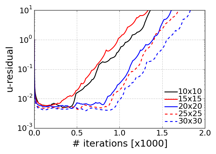
Here, the test has conducted with Re = 10,000 such that the equation almost goes to Euler equation. We can expect that numerical solution will be unconditionally unstable because our employed finite difference is done with central differencing. The test shown below proves this. On the other hand, the effect of grid spacing on the unstable solution’s temporal evolution is clarified. Even though all the cases go to unstable solution after all, the onset of amplified numerical instability appears at different location in iteration number.
Effect of grid spacing on the temporal evolution of axial velocity residual. (Re = 10,000)
Maximum time step
In this code, the variable time step method is used to maintain stable numerically. Therefore, the code does not run with constant time step. The maximum time step test is performed with different set of Courant number condition. The grid spacing is fixed with 20x20 to have fast running of simulation.
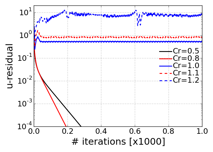
As described earlier, the current project is to set the numerical time step variable according to the stability criteria taking Courant number into consideration. The Courant number is essentially based on convective velocity that transport the flow quantities that may propagate the numerical signal waves. Since the current system of equation is based on incompressible flow equation, the convective velocity is simply equivalent to the local velocity components at every node points. As we discovered the numerical instability characteristics with Burger’s equation, the required Courant number is to be less than 1.0. In this regard, the time step experiment in this section seems to well satisfy this requirement. Having Courant number less than 1.0 shows well stabilized solution as we observed from the above plot.
Since the current code is featured with variable time step, single value of time step can be representative of the required time step. Instead, we employed a certain numbers of Courant numbers as listed below. The representative time step value is chosen when the temporal iteration reaches 100.
Courant # dt at 100th iteration 0.5 0.038791 0.8 0.061655 1.0 0.064686 1.1 0.063479 1.2 0.072822